
Changing Sea level budget and Semi-Empirical models
It is expected that the balance of the sea level budget will change in the future as the slow giants of the ice sheets awaken. This has been leveled as a criticism of semi-empirical models. For that reason people sometimes (wrongly) argue that “the data used to derive the model, do not contain the effect of the processes, which we expect in the future to dominate”. Here I demonstrate that this argument is flawed using an extremely simplified conceptual model.
Featured image from Ali Almossawi’s Illustrated Book of Bad arguments:
Conceptual Model:
I assume that the contributions from steric, glaciers and icesheets are all responding linearly to global average warming. This is the model:
stericRate   = (T-mean(T<sub>1940:1960</sub>))/700
icesheetRate = (T-mean(T<sub>1950:1970</sub>))/300
glacierRate  = (T-mean(T<sub>1880:1900</sub>))/2000
where T is global mean temperature in degC. This means that the rate of total sea level rise will also be proportional to warming (see footnote 2). Thus in this idealized world we know that the Rahmstorf (2007) model is 100% correct.
For convenience I use EC-EARTH model temperatures as T (as they cover both past and future).
Please note this model is not designed to be realistic but just demonstrate that the premise of the argument presented above is flawed.
Footnote 1: Why three different baseline temperatures?
In the conceptual model there are three different baseline temperatures / equilibrium temperatures. One might ask how realistic is that.
In the real world the three contributors have different sensitivities and different response times, and the model would only be an approximation. The slow giants of the ice sheets have a long response time compared to the glaciers. This means that at the end of the Little Ice Age then we must expect the glaciers to be much closer to equilibrium than the ice sheets which will still have some memory of the medieval warm period. I.e. we will expect that the glacier equilibrium temperature would be colder than the equilibrium temperature for the ice sheets. This is the motivation for choosing different baseline temps in the model.
We can argue about how much memory each contributor exactly has, but the point is that their response times are different, and in turn that different baselines are to be expected.
Footnote 2: Equivalence with Rahmstorf 2007:
GSL_Rate = stericRate + icesheetRate + glacierRate
= (T-T1)_a1 + (T-T2)_a2 + (T-T3)_a3
= T_(a1+a2+a3) - T1_a1 - T2_a2 - T3_a3
= (T-T)_a
where
- T1=mean(T1940:1960)
- T2=mean(T1950:1970)
- T3=mean(T1880:1900)
- a1=1/700
- a2=1/300
- a3=1/2000
- a = a1+a2+a3
- T0 = (T1*a1 + T2*a2 + T3*a3)/a
Output
The model output shows that the dominating contributor changes between the 20th and 21st centuries and yet we know that in this idealized world the Rahmstorf 2007 model works. This demonstrates that this particular argument against semi-emprical models is fundamentally flawed. Semi empirical models of sea level rise can be perfectly consistent with a shift in dominance.
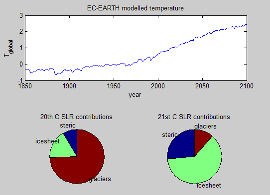
*Note only temperature is output from EC-EARTH. The pie charts are based on the conceptual model on this web page.
No good data on past ice sheet contribution.
Finally, there is very little data on past ice sheet contributions, and that is another reason why I have serious problems with the argument “the data used to derive the model, do not contain the effect of the processes, which we expect in the future to dominate”. To make this argument you have to know know how ice sheets behaved throughout the 19th and 20th centuries. How could they possibly know this?
Matlab example:
T=load('global_tas_Amon_EC-EARTH_rcp45_ave.dat');
t=T(:,1);
T=mean(T(:,2:13),2)-286;
plot(t,T)
stericRate=(T-mean(T(ismember(t,1940:1960))))/700;
icesheetRate=(T-mean(T(ismember(t,1950:1970))))/300;
glacierRate=(T-mean(T(ismember(t,1880:1900))))/2000;
close all
subaxis(2,2,1,1,2,1,'sv',.2)
plot(t,T);
title('EC-EARTH modelled temperature')
subaxis(2,2,1,2)
ix=find(ismember(t,1900:2000));
rates=mean([stericRate(ix) icesheetRate(ix) glacierRate(ix)]);
pie(rates*1e8,{'steric' 'icesheet' 'glaciers'})
title('20th C SLR contributions')
subaxis(2,2,2,2)
ix=find(ismember(t,2000:2100));
rates=mean([stericRate(ix) icesheetRate(ix) glacierRate(ix)])
pie(rates*1e8,{'steric' 'icesheet' 'glaciers'})
title('21st C SLR contributions')
colormap jet