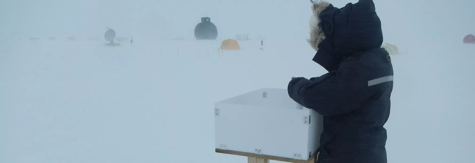
Greenland Monthly Accumulation Maps (1960–2022)
Regional climate models give us beautiful, spatially complete maps of Greenland snowfall. Millions of radar, firn-core and snow-pit measurements tell us where those maps are wrong. How do you get the best of both?
The problem
Snowfall is the only mass input to the Greenland ice sheet, and ice-sheet models need it as a gridded, spatially complete field. In practice that means RCM output. But RCMs carry biases that vary in space and time, from unresolved orography, simplified cloud microphysics, and boundary forcing that is less constrained in earlier decades. And different models disagree about where the snow falls.
Meanwhile, the observational record has grown enormously. The SUMup database now holds more than two million accumulation measurements from airborne and ground-based radar, firn cores, snow pits, stakes and more. The catch is that these observations are messy from a model’s point of view: they’re points rather than grid cells, they span anything from a week to several years, and many have dating uncertainties of up to a year. Simple point-by-point comparisons waste most of that information.
The approach
Our idea is to correct the model in a reduced space rather than grid cell by grid cell. We decompose each model’s monthly accumulation into a mean field, a seasonal climatology, and the leading EOFs with their principal components. We then fit a small set of adjustment coefficients to SUMup: one shifting the mean, one scaling each EOF pattern, one scaling the climatology, and one scaling each PC time series. With 10 EOFs, that’s 22 parameters to describe the bias of an entire ice sheet over six decades.
The EOFs aren’t meant to be interpreted physically here. They’re simply a smooth, low-dimensional basis that lets sparse observations inform the whole field. A few details make the fit robust to the realities of SUMup. Each observation is compared with the model over its actual measurement window, with dating uncertainty represented as a Gaussian weighting. The time-dependent coefficients are regularized towards “no adjustment”, with the strength chosen by cross-validation in which all data from the same core, pit or radar horizon stay in the same fold. A robust loss function limits the influence of outliers.
We applied this to HIRHAM5, MAR 3.14, RACMO 2.4p1 and CARRA.
What we found
Every model has significant biases, but they look very different. HIRHAM is biased low across most of the ice sheet, while CARRA is biased high by about 10 % against the observations. MAR and RACMO look nearly unbiased in the ice-sheet mean, but that hides compensating regional errors: positive biases in the south and negative biases further north. All three of HIRHAM, MAR and RACMO underestimate accumulation in the cold, dry northern interior, locally by 30–50 %.
The south dominates the net bias in all models, in the south-east for HIRHAM and MAR and in the south-west for RACMO and CARRA. That’s no surprise to anyone who has looked at orographic precipitation along the south-east margin, but the dense radar coverage lets us quantify it in places earlier ice-core-based evaluations couldn’t reach.
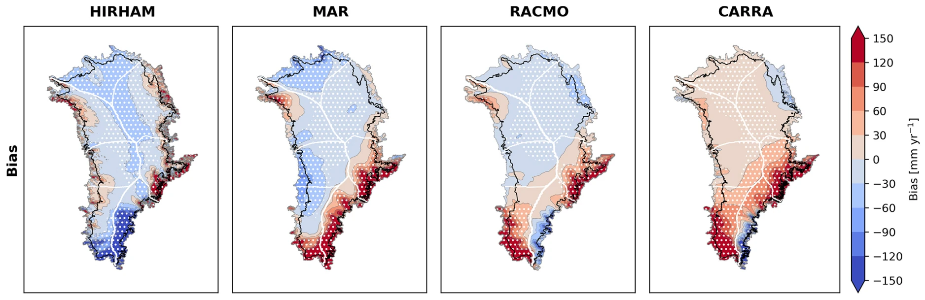
Mean accumulation bias of HIRHAM, MAR, RACMO and CARRA, shown as the original model minus the bias-adjusted field (mm per year). Red means the model accumulates too much snow, blue too little.
After adjustment, the models converge where the data are dense. In the accumulation zone, inter-model spread in mean accumulation drops by 68 %, with MAR, RACMO and CARRA landing within a few mm per year of each other at around 390 mm w.e. per year. In the sparsely sampled ablation zone the opposite happens, and the spread grows. The correction can only be as good as the observations behind it.
Both the original and adjusted fields show a striking east-west contrast in trends and temperature sensitivity: positive in the east, negative in much of the west, with the strongest trends in the south-east.
Why it matters
A 10 % accumulation bias sounds modest, but over a century it adds up to around 8000 Gt, or about 25 mm of sea-level rise. An 80 Gt per year SMB error is roughly equivalent to a 1°C warming bias, which is not small compared with estimated thresholds for long-term Greenland mass loss. Spatial pattern matters too: accumulation errors get absorbed into the calibration of ice-flow parameters, so getting where the snow falls right matters for ice dynamics, not just for the mass budget.
Caveats
The adjustment is sensitive to methodological choices such as how many EOFs to retain. Radar dominates the fit, so any systematic radar bias, including density assumptions, propagates into the result. And with very few monthly observations, the seasonal corrections are much less robust than the annual ones. More density-independent snow-water-equivalent observations, especially in the ablation zone and the south, would help most.
What’s next
Because the method works in EOF space, it suggests a route back in time. The PCs correlate with the NAO, Greenland blocking and sea-ice cover, and if we can model them from climate indices and proxies such as ice cores and tree rings, we can build spatially complete reconstructions of past accumulation. That’s the topic of an ongoing PhD project.
The bias-adjusted fields for all four models are on Zenodo, together with prefiltered SUMup data and minimal working code. The code can be applied to any gridded accumulation product.