
Sea level, the moon, and Frankenstein
Jens Morten Hansen (JMH) and co-authors have recently published a study where they use sine-regression to fit 5 oscillations plus a linear trend to a 160-year sea level record from waters near Denmark (a stack of local GIA corrected tide gauge records). They then observe that the sines-plus-trend model correlates highly with the record it was fitted to, after applying a 19-year moving average. This should be unsurprising as the procedure guarantees high correlation, regardless of input data (see figure). This result is clearly not significant in any meaningful sense of the word.
After having tuned their model to fit the data, they proceed to post-rationalize the fitted model frequencies in terms of the nearest half-multiples of the lunar nodal cycle (18.6 years). I use the word “post-rationalize” to highlight that their new hypothesis is formulated in order to explain their first insignificant result. Again, this key result is clearly not significant. You can postulate any similar set of frequencies, and you would still get high correlation. This is illustrated in the figure on this page where we show how sea level can be ‘predicted’ using the orbital periods of five exoplanets.
It is therefore not surprising that it has been hard to get this study published. After multiple rejections, it was eventually published in Journal of Coastal Research. JMH then began to publicize it in primarily danish media. Here are some of the headlines it generated:
- **Scientific censorship in the name of climate | **“Forskningscensur i klimaets navn” (forskeren)
- Danish scientists: Humans not to blame for higher sea levels | “Danske forskere: Mennesket er ikke skyld i højere vandstande” (Berlingske)
- **Moon-cycle gives exaggerated numbers for sea level rise | **“Månecyklus giver overdrevne tal for havstigning” (Ingeniøren)
- **The effect of the moon on sea level | **“Månens effekt på havspejlet” (Weekendavisen)
- **No detectable effect on sea levels from global warming | **“Ingen påviselig effekt på havniveauet af global opvarmning” (aktuelnaturvidenskab)
This persistent push for publicity have prompted us to voice our critical concerns regarding this study. No, this is not a case of scientific censorship. This study has fundamental flaws and it is simply not convincing.
[Update: Our criticism is now out in Aktuel Naturvidenskab and republished on videnskab.dk. Lise Brix from Videnskab.dk followed up with a thorough piece where they interview outside experts. Schmith et al. (2016) has written a formal critical comment to the journal.]
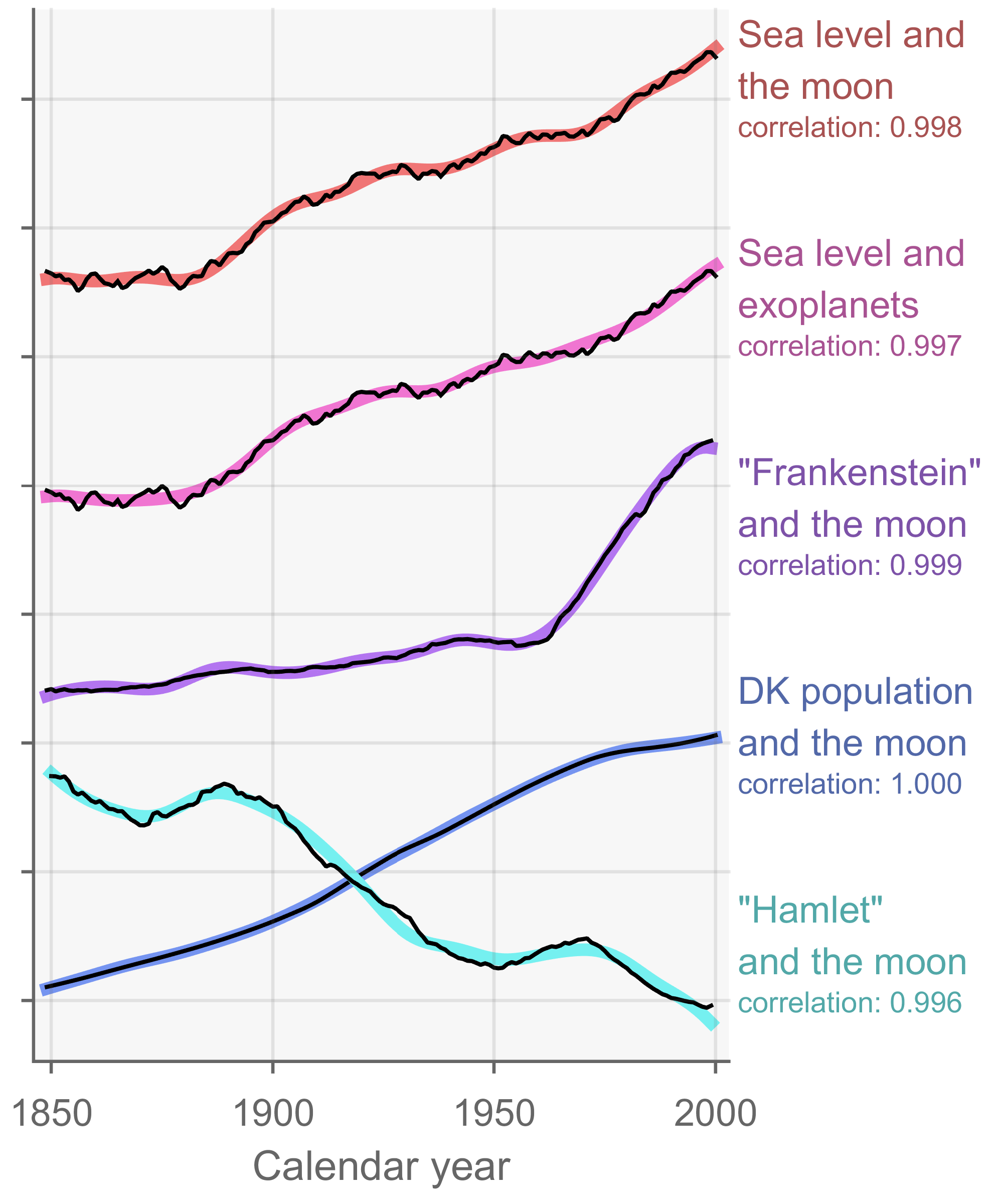
The sea level series can be fitted using a sum of five multiples of the nodal cycle plus a trend, but that does not mean there is a causal relationship. Virtually any time series can be fitted using the exact same set of frequencies, and that any similar set can fit the sea level series. We illustrate this by ‘predicting’ time series of frequencies of the words ‘Frankenstein’ and ‘hamlet’ in books and the population in Denmark using the nodal cycle, and by predicting sea level using the periods of five exoplanets.
Our criticism - over fitting
We wrote a critical comment highlighting the flaws in their analysis. It can be found here (in danish). We demonstrate by example the non-significance by showing how you get high correlations regardless of data set, and periods used (see figure).
The plot on this page shows how we can fit pretty much any time series using the exact same lunar frequencies they used in their study. We illustrate this using data for the population in Denmark over time, and the frequency of the words “Frankenstein”, and “hamlet” in books over time. We can also predict sea level using the orbital periods of exoplanets. The point is that high-correlations are guaranteed even when there clearly is no causal link.
The basic issue is over-fitting: Their statistical model has 17 degrees of freedom (5 periods, 5 phases, 5 amplitudes, 1 trend, 1 constant). They test the quality of the resulting fit against 19-year moving averages of a 160-year series. There is at effectively 8-9 independent points in the smoothed series (naive estimate). Of course it will fit with a high correlation coefficient.
_“With four parameters I can fit an elephant, and with five I can make him wiggle his trunk” - John von Neumann
Mayer et al. (2010) put Neumann’s statement to the test and fit a cycle model to a drawing of an elephant. The model is remarkably similar to JMHs sea level moon model, albeit with fewer free parameters and with additional periodicity constraints.
Post-hoc rationalization of an insignificant result
JMH and coauthors were struck by the high-correlation, and felt they needed a causal explanation. Our examples show that there is absolutely no need for an explanation as their procedure guarantees high correlations even when there is no causal link. They then come-up with what I call the lunar nodal resonance hypothesis where all sea level variability is explained by the moon. I see this as a post-hoc rationalization of a (very) insignificant correlation, and I am not convinced.
Armed with their new nodal resonance hypothesis, they reformulate their model with the frequencies rounded to nearest half-multiple of the nodal cycle. They then re-optimize all the remaining parameters and ’test’ whether the nodal resonance model also can fit the data. We show that this is a poor test as it is also guaranteed to give a positive result.
Personally I also think the nodal resonance hypothesis is physically far-fetched. I don’t have a problem with the nodal cycle having a detectable effect on sea levels, but he is also arguing that multiples thereof have a large significant effect on winds (and AMO / NAO). That is quite a mental leap. In his own words:
_“Additionally, we have [in Denmark] documented additional cyclic oscillation with a period length of 76 years. This oscillation implies, by all accounts , that we are entering a period of more easterly wind” _- Jens Morten Hansen (translated by me, original here)
Other notes
JMH presents the iterative hand-tuning of parameters as a strength, presumably because there is no incomprehensible mathematical ‘magic’ going on. I see the manual iterative procedure as a weakness. The manual hand-tuning means it probably will be impossible to exactly replicate the results. Another problem is that the iterative search is not guaranteed to result in a globally best-fitting solution. (Further, an automated procedure would also facilitate a Monte Carlo significance testing against a reasonable null.)
The paper makes no serious attempt at validation. They could have done a cross calibration / validation exercise. The could also have compared their statistical hind-cast to GIA adjusted versions of the longer tide gauge records from Northern Europe.
Their explanatory model is entirely tidal, and thus leaves no room for climate change to have any impact on sea level. This is regardless of whether it is natural or anthropogenic climate change. -But we know how glaciers have retreated globally (Zemp et al. 2015), and therefore must have contributed to sea level rise over this period. Clearly, the global mountain glacier retreat cannot be forced by the lunar nodal oscillation. This inflexibility of their statistical model exposes a fundamental problem.
In a radio show from the danish national broadcasting company (DR), JMH lets us know that he and a like-minded swede tried to push the story to a major Swedish newspaper. It was rejected with a note that the newspaper never accepted letters opening with references to the Emperors new clothes. I find that particular reference ironic.
A google search reveals that JMH is on the scientific board of klimarealistene in Norway. They have the motto: “it is the sun that drives climate”, and their logo looks like a sun and a sine wave. Mörner is also on the board, and I wonder if he is the like-minded swede.
There is a tendency to see cycles everywhere. JMH claims that the AMO has a clear period of 74 years, and that NAO has a clear period of 56 years (Link in Danish). I strongly dispute that these two indices have ‘clear’ periodicities on those wavelengths. Here’s a graph of the NAO - can you spot the “clear” 56 year cycle?
JMH believes that it is consensus thinking and scientific censorship in the name of climate which made it hard for him to publish his ‘bomb-shell’ study (See forskeren.dk). Well, the type of cycle fitting in JMHs paper is also unconvincing to climate change skeptics: Here’s Willis Eschenbach using the term “cyclomania” with respect to a somewhat similar analysis by Scafetta. Nobody can argue that Willis is part of the climate change consensus (see exhibit a).
“I sat one evening in my laboratory; the sun had set, and the moon was just rising from the sea; I had not sufficient light for my employment, and I remained idle, in a pause of consideration of whether I should leave my labour for the night or hasten its conclusion by an unremitting attention to it. As I sat, a train of reflection occurred to me which led me to consider the effects of what I was now doing.” Mary Shelley 1818
Sources
The data in the figure comes from these sources: Sea level digitized from JMHs paper. Word frequencies from google ngrams. DK population from statistikbanken.dk. exoplanet periods from openexoplanetcatalogue.com. The particular datasets were chosen based on these criteria: 1) same temporal coverage as JMHs sea level series. 2) could not be argued to be causally linked to the nodal cycle. Elephant wiggly trunk code can be found here.
The new title of this page is credited to a tweet by Sou.
Update: I made a guerrilla poster for EGU 2016 based on this page.